FLood2: Turbulence Characterization with the Lambda-2 Criterion

As I wrapped up my undergrad in chemical engineering and computer science, I had the opportunity to work as an undergraduate researcher in a computational fluid dynamics (CFD) group.

This post is meant as a brief, 5-minute overview of that work. It highlights the motivation behind the criterion, the algorithm I developed, and some key results from applying it to turbulent flows.

This was my first exposure to true distributed computing. In the end, I have a novel contribution to the CFD field, and an algorithm that distributes across hundreds of cores.

Criterion Background

Identification and subsequently visualization of vortical structures is fundamental for characterizing coherent motions within complex flows. Most detection methods are based on the velocity-gradient tensor, J, including the Lambda 2 method, which is the backbone of the algorithm being showcased in this section.

This transformation matrix can uniquely decomposed into two physically distinct components: a symmetric strain-rate tensor, S, and an antisymmetric rotation-rate tensor, Ω:

Physically, the symmetric strain-rate tensor represents fluid deformation associated with stretching and compression without rotation, whereas the antisymmetric rotation-rate tensor represents the pure rotational motion of the fluid.

Under the assumptions of incompressibility, negligible viscous effects, and negligible irrotational straining, the Navier-Stokes equations simplify in a way as to allow the second-order tensor combination:

to directly correlate with the existence of a local pressure minimum, which is a necessary but not sufficient condition for a vortex core.

The symmetric strain tensor admits only real eigenvalues, and thus positive and real eigenvalues for the square. Conversely, the antisymmetric rotation tensor results in up to two imaginary eigenvalues, which become negative and real when squared. So, the combination of the squares of these two tensors results in a symmetric tensor whose eigenvalue signs are determined by whether the stress or rotation eigenvalues had the greater magnitude.

By taking the eigenvalues and sorting them:

with

the second eigenvalue yields the criterion used for vortex identification, which is the result of comparing the weaker strain value with the rotation.

The magnitude of the second most negative eigenvalue is directly proportional to the strength of rotation relative to strain; a more negative signifies a stronger vortex structure. However, the practical implementation of the criterion typically involves visualizing isocontours of its scalar field. Determining the appropriate cutoff threshold for these contours is completely qualitative, and common methods to select this threshold include subjective visual inspection, or a fixed volume fraction of the fluid domain for comparing multiple flows. Both approaches introduce substantial variability and limit the criterion’s effectiveness in quantitative turbulence characterization or comparing trends across flows.

Algorithm Development and Analysis

To address the inherent subjectivity and limited quantitative capabilities of the conventional method, a flood-fill-based vortex characterization algorithm termed FLood2 was developed. This algorithm evaluates vortex structures across a range of threshold values, providing quantitative metrics such as vortex size, quantity, and location.

The FLood2 algorithm initially computes the scalar field from the simulated velocity field using the standard criterion. This scalar field is computed at mesh vertices using the Nektar++ post-processing utility. To facilitate subsequent quantitative analysis, the values initially defined at mesh vertices are interpolated to cell centers by taking the arithmetic average of the values at the cell’s eight vertices.

Additionally, the quantitative analysis requires computation of the cell volumes. For fully structured hexahedral meshes, each hexahedral cell volume is calculated by decomposing the cell into a set of tetrahedra whose volumes are computed via the scalar triple product. Given the consistent vertex ordering guaranteed by the VTK standard, this decomposition and volume computation is straightforward and unambiguous.

The core of the FLood2 algorithm uses a breadth-first search (BFS) flood-fill. First, an adjacency map is created, identifying neighboring cells based on the number of shared vertices. In structured hexahedral meshes, two cells are neighbors if and only if they share exactly four vertices.

For each cutoff in the range, the BFS process explores contiguous cells whose values lie below a specified threshold, marking each group of connected cells as a distinct “island” or vortex region. For each identified island, the algorithm records quantitative properties such as the total volume occupied by the vortex and its volume-weighted centroid position.

Since FLood2 must examine every one of the cells for each of the sampled thresholds, its overall computational cost scales as , where is the total cell count in the mesh and is the number of threshold values investigated.

Running in Parallel

A significant advantage of the FLood2 algorithm is its inherent parallelizability. First, the sampled thresholds can be trivially distributed, since each threshold’s flood-fill is entirely independent from the others. This gives embarrassingly parallel scaling in the threshold dimension.

To achieve spatial parallelism within a threshold, the computational domain can be partitioned into non-overlapping subdomains by graph partitioning. Each subdomain, or rank, is assigned to one process or thread. Within its subdomain, the worker only performs BFS on its owned cells, and assigns unique island IDs. This generates a set of local vortex islands labeled independently in each partition. Because subdomains are disjoint, these BFS traversals can be done concurrently without race conditions.

Because vortices can cross partition boundaries, local islands that touch across ranks must be merged. This is done by recording an equivalence relation: if a boundary cell in rank A’s island a is adjacent to a boundary cell in rank B’s island b, then we record the equivalence:

In other words, these islands are part of the same global vortex if they contain any face-connected cells. These equivalences form a graph connecting local island IDs across ranks. To resolve equivalences, a distributed union-find algorithm is applied. This process assigns a single global component ID to every island such that islands spanning multiple partitions are stitched into one vortex. Finally, each rank contributes its partial volume and centroid moment sums for its owned cells, keyed by the global component ID; a global reduction then produces the total volume and centroid of each stitched vortex.

SZ Geometry Turbulent Flow Characterization

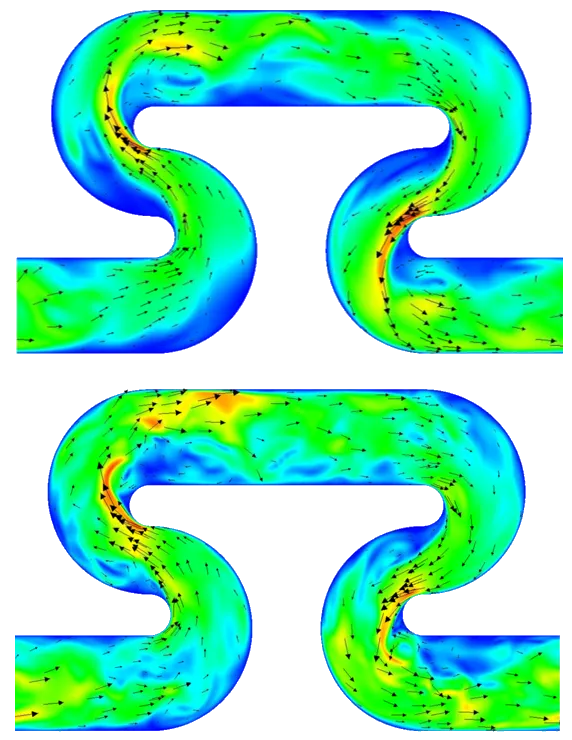
This algorithm was tested on a turbulent flow in the SZ geometry. Based on the velocity magnitude contours of cross-sectional slices, Reynolds numbers of 500 and 1000 create enough turbulent structures for a proper analysis.

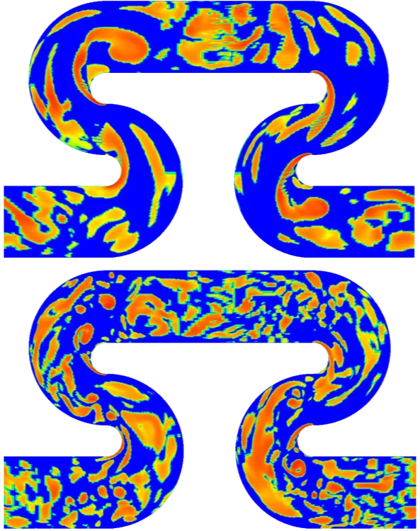
Likewise, after filtering out all positive regions and examining the cross section contour plot of the log of the criterion, a distinct shift in the vortical structures can be seen, including significant changes in vortex sizes, distributions, and quantities.

Quantitative Analysis using FLood2 Algorithm

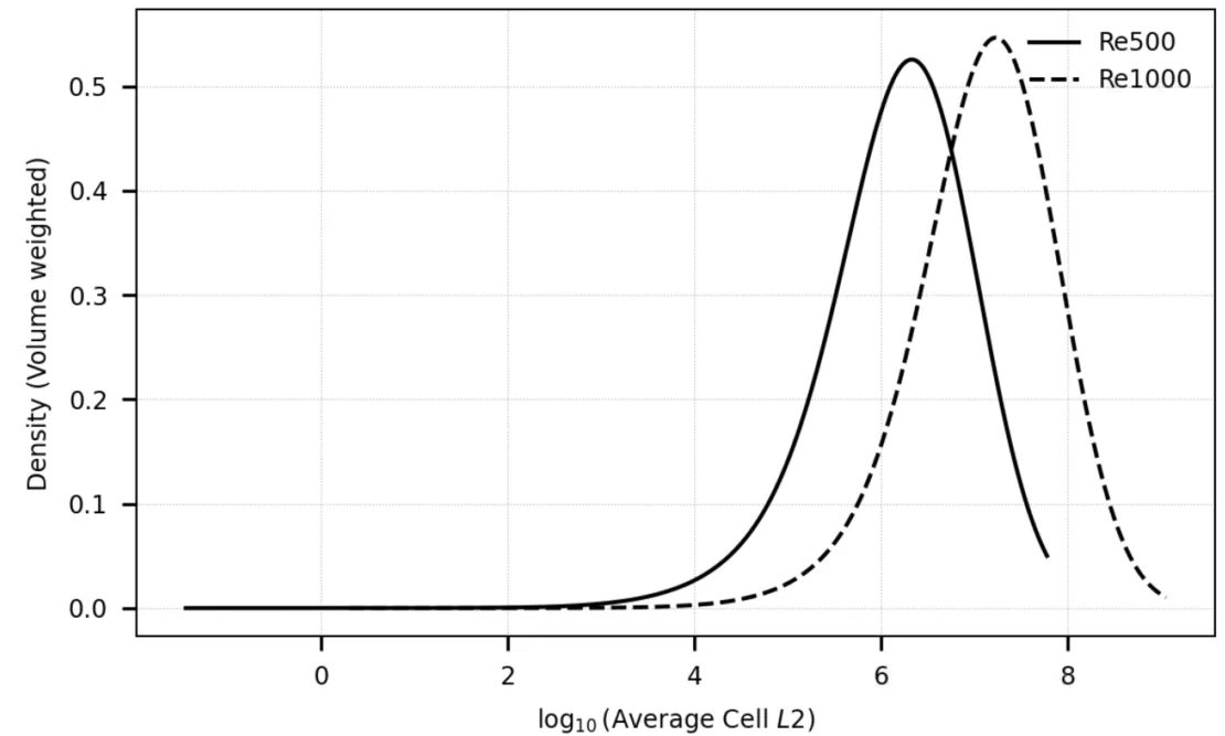
Initial distributions of volume-weighted values offered limited insight as they spanned many orders of magnitude. However, once regions dominated by strain were excluded and the remaining values transformed using the logarithm of their absolute values, a clear log-normal distribution emerges. This demonstrates that higher Reynolds number flows produce stronger vortices, showing an approximately 20% increase in average vortex intensity on the log scale when doubling the inlet velocity.

The skew in the distributions reflects the fact that large, high-energy eddies fragment into smaller structures more quickly than the reverse process, so very strong vortices are rarer, suppressing the upper tail. A slight reduction in standard deviation was also noted at Re = 1000. Most importantly, these distributions help decide the range of lambda values to sample FLood2 across; in this case, a range of was selected, sampled at 20 evenly spaced intervals.

Analyzing the relationship between the average vortex volume and threshold indicates that increasing the Reynolds number results in a smaller average vortex size, despite the occupying a larger fraction of the flow field at any given threshold. This behavior occurs because higher Reynolds numbers generate small vortices in regions previously devoid of turbulence at a given time, as well as fragment large vortices into multiple smaller vortices.

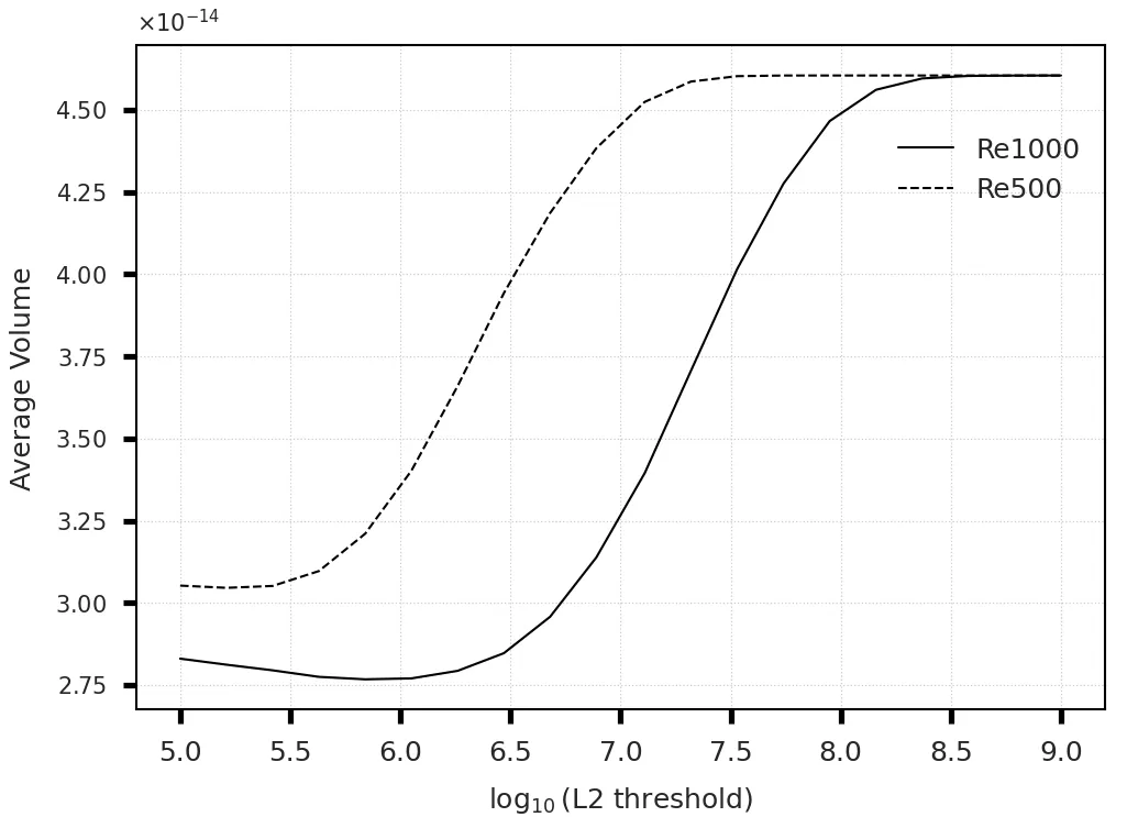
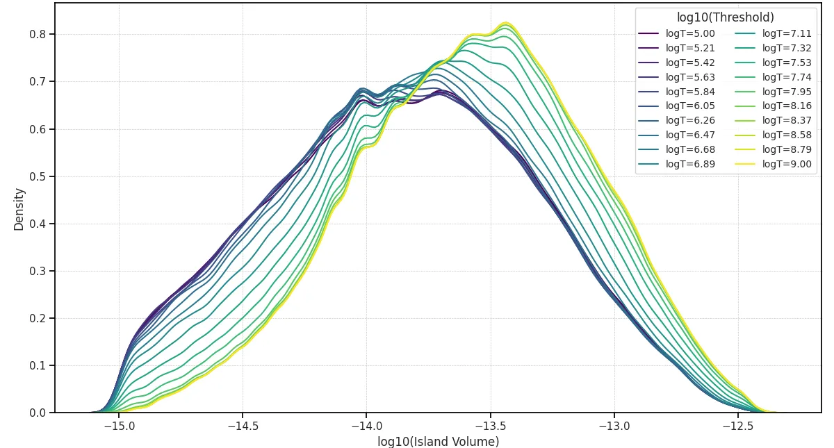
Looking at the distribution of vortex volumes within a single Reynolds number rather than simply tracking the average across Reynolds numbers also provides valuable insight. The distribution of vortex volumes at Re = 500 shows a progressive shift toward larger average sizes as the cutoff threshold increases. Although initially counterintuitive, this is consistent with the turbulent energy spectrum, where most kinetic energy comes from low-frequency large-scale eddies, so by filtering for high-intensity we naturally isolate fewer, but bigger, coherent vortices.

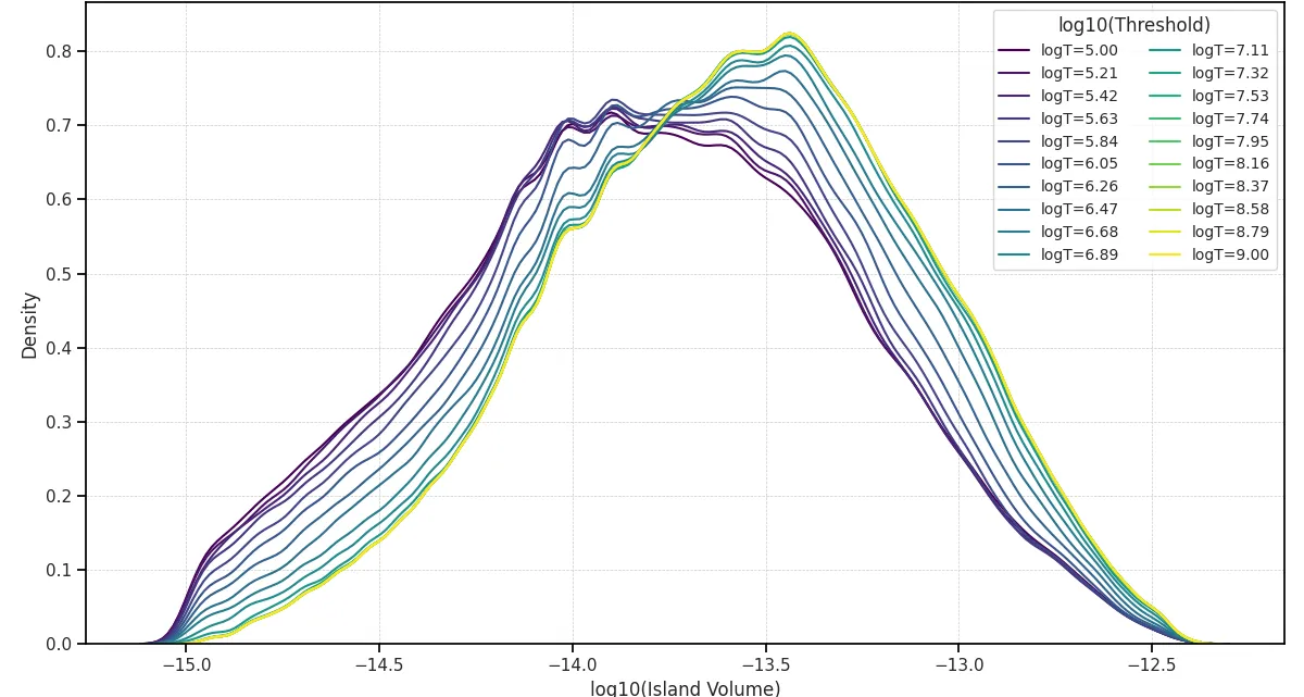
Increasing Reynolds number from 500 to 1000 altered the vortex size distribution by broadening and shifting it towards larger vortices at lower thresholds. At the stricter thresholds, the distribution remained largely unchanged, suggesting that the increase in flow intensity at Re = 1000 primarily affected weaker vortices. Higher Reynolds numbers would likely further shift the distributions towards larger vortices even at stricter criteria.